Saturday, June 3, 2017

Applications: Projects requiring solutions of systems

Solving systems of equations


Nodal analysis of circuits - Uses systems of equations to find the current through each loop of a circuit including batteries and resisters.  Nodal analysis creates linear equations using Kirchhoff's Laws of junctions and paths.  This is a popular project for students who have studied some physics.  One value of this project is the ability to create overdetermined, consistent systems of equations, which helps students understand rows of zeros in the RREF form of augmented matrices.  This article on Nodal Analysis of Electric Circuits has a clear explanation.

Loop analysis of circuits - Uses systems of equations to find the current through each loop of a circuit including batteries and resisters.  Loop analysis creates linear equations using Kirchhoff's Laws of loops.  Again, a popular project for students who have studied some physics and also has the opportunity for overdetermined, consistent systems.  Equivalent in results to nodal analysis, this could be combined or assigned separately.  This article on Loop Analysis of Electric Circuits has a clear explanation.

Curve fitting - Using systems of equations a student finds the coefficients of a polynomial of degree n - 1 to fit n points.  I don't think of this as a juicy application that gives the student an appreciation for how linear algebra is used in the world.  Fitting an n-degree polynomial to m points using least squares or other methods is more likely to happen.


Thursday, June 1, 2017

Applications: Projects using vector spaces

Inner product spaces


Curve fitting using least squares - Uses matrix multiplication, inverses, and equations to find coefficients of a curve that fits a set of points.  I have three misgivings about curve fitting with least squares: it can be done without any understanding, it is not representative of least squares problems in general, and the various spaces involved confuses the issue.  Taking the last point first, the problem involves points in 2D or 3D space, matrices in n x k space where n is the number of points and k the terms of the curve being fit, and coefficients that live in k-space.  If we are trying to fit a line, the coefficients are 2D, but that 2D space is not the 2D space of the original points.

If a student is assigned this project without have learned about projections, they can do the calculations anyway, since they just require matrix multiplication and solving systems of equations.  The process of setting up the matrices does not promote deeper understanding of inner product spaces, and so if the student is going to fit curves, they might as well use Excel, which also doesn't deepen their understanding of linear algebra.

Finally, if a student learns least squares in this way, then they have difficulty transferring this concept to the solutions of noisy systems using least squares and don't think of least squares as a method of approximating solutions, but rather of fitting curves.

Friday, May 26, 2017

Applications: A list of projects using matrix operations

Matrix Operations

I've just finished teaching Linear Algebra twice since the beginning of the year, and I'll be teaching it again in the fall. It is time that I cleaned up my applications list and updated the project files. Since I am enumerating them, I might as well do it here. Here is part 1 on matrix operations.  Others may be added later.

Seriation in archaeology - Uses incident matrices, matrix multiplication and transposition, and the properties of symmetric matrices to determine relative ages of sites with common artifacts.  I haven't used this in my classes yet, but there seem to be some good resources available including "Some problems and method in statistical archaeology," David Kendall, World Archaeology, 1969, which is available in JStor.  It also appears in Gareth Williams Linear Algebra with Applications.

Color manipulation in images - Uses matrix multiplication to alter colors in the RGB scale.  This article by Paul Haeberli describes the 4x4 matrices needed to modify colors, including offsets.  I haven't used this in class yet, but I could see this as a good project to have students work in Mathematica.  It also is a companion for transformations in 3D graphics, which also use 4x4 matrices.  The ability to use matrix multiplication to add vectors is common to both areas.

Image color conversion - Uses matrix multiplication to convert from, say, RGB to YIQ, color models.  I haven't used this in class, but it shows up in Gareth Williams Linear Algebra with Applications. This article by Ford and Roberts describes a bevy of color models, and it seems that only some conversions are linear.  Without a way to test whether the color conversion is correct, I don't see this as an interesting project. However, maybe Mathematica can render the other color models.

Transformations in 2D graphics - Uses matrix multiplication to apply rigid and non-rigid transformations to images.  May or may not use projective coordinates, depending on whether translations are allowed.  Resources abound.

Projection of 3D images onto the plane - Uses matrix multiplication to project 3D images onto the plane given the coordinates of the image and the location of the viewer.  Uses projective coordinates.  I use a paper written by Jeanie Mullen, one of my honors students.  This project has worked best for students with programming backgrounds.

Two-port in an electrical circuit - Uses matrix multiplication to describe the change in voltage and current through a two-port or a series of two-ports.  A simple application of Ohm's law that creates two linear equations that can be described using matrix multiplication.  The equations relate the input current and voltage to the output current and voltage.  This Wikipedia article has a table of many transmission matrices and their effect.

Wednesday, May 24, 2017

Applications: A list of projects using eigenthings

Eigenthings

Gould's accessibility index in a network - The process uses a modified adjacency matrix and the components of the eigenvector associated with the dominant eigenvalue. Students find this approachable and adaptable.  Applications to historical geography, air traffic.

Discrete dynamical systems - Using linear algebra to study discrete dynamical systems comes in several flavors.  Here are some projects that students find interesting and that differ from each other enough that they feel they are not repeating someone else's project.


  • Difference equations and the Fibonacci sequence - Using eigenvalues to write the product of the nth power of a diagonalizable matrix and an initial vector allows one to write a closed form for a recursive formula.  Matrices of size 2x2 are needed to write the closed form of the nth Fibonacci number, but students can easily move from there to the closed form of 3rd and 4th order difference equations.  This project is always chosen by some student even though it is not applied to a real-world situation.

Monday, May 22, 2017

Applications: A list of projects using matrix inverses

Matrix Inverses


I separate these projects from those other using matrix operations, because I make a clear distinction between forward and inverse problems in my classes.

Cryptography - These projects come in two varieties: using modular arithmetic and not.

  • Matrices with |determinant| = 1 - Uses matrix multiplication to encode a matrix and multiplication of the inverse to decode.  Any matrix with determinant 1 or -1 will result in an inverse with integer components.  Students tend to be drawn to these projects, but sometimes I find it hard to push them further, such as requiring them to create their own encoding matrices, etc.  Resources abound.
  • Modular arithmetic and row reduction - Uses matrix multiplication in modular arithmetic to encode and decode a message and row reduction in modular arithmetic to find the inverse.  This is not that the decoded matrix is read using mod 26, but rather that the matrix operations are done with, say, mod 37.  This project requires a little more tenacity on the part of the student, and this article by Keith Conrad discusses inverses of matrices under modular arithmetic.


Saturday, July 31, 2010

Interesting property of the inverses of Magic Squares

I’m a nerd. I freely admit it. Sometimes I see a result in mathematics that I think is fun, even if it is not immediately useful. I intended for this blog to be about applications of linear algebra, and by that I mean useful, if not a little esoteric, applications; applications that are juicy and interesting and have good visuals. Although the abstract applications of linear algebra to theoretical areas of mathematics are useful to someone, they do not have the hands-on feeling that I want. However, the nerd in me finds some abstract ideas sexy enough to include in this blog. The following is one of them. Although there is a connection between this idea and Magic Squares, which have constant row sums, I don’t see an application right off. If you know of one, please let me know.

Theorem (already this post looks different than usual ‘cause it has a theorem):
If an invertible matrix A had constant row sums of k, then the inverse of A has constant row sums of 1/k.

Proof (Oh, no.  A proof.  Just when this blog looked like it was just fun stuff):
Let A be an m-by-m invertible matrix with constant row sums of k. Let B be the inverse of A.  Now, AB = I and the diagonal elements of I are all 1.  Note that I has a constant row sum of 1.  Hmmm.  Let

             (1)
be the elements of I.  Then
                  (2)
is the sum of the elements of row i of I, and
              (3)
is the sum of the elements of row n of A.  Now, write the elements of a row of I = BA as the sum of products of elements of A and B:
             (4)
Now, we're ready to put this all together.
Thus,

         (5)

but the right-hand side of (5) is the sum of row i of B

It seems like a trick, and in a way it is, but the trick is legit.  What we have done is started with the sum of row i of I, written it in terms of the elements of A and B, and then seen that we could factor out the elements of B leaving row sums of A.  To help you understand this, carefully write the elements of a general 3-by-3 BA in terms of the elements of B and A.  Now, sum one of the rows of BA and rearrange so you can factor out the various elements of B.  The sums of the elements of A left will each be a row sum.  This wouldn't be a proof in general, but it should help you understand what is happening in that sum-switching step of the proof, and that it works because the elements of a matrix product are sums and then we sum a row of sums, and the terms within these two sums can be conveniently rearranged.

Questions

  1. We started with an invertible A with constant row sum.  What if A had constant column sum of k instead of row sum?  Will the inverse of A have constant column sum of 1/k as well?  How would the proof go for that?  This would be a great exercise in working with sums and indices.

  2. This proof will not work if the constant row sum is k = 0.  Can a matrix have an inverse if k = 0?   If k is not zero, are we guaranteed that A is invertible?  Can we determine if a magic square is invertible by the row sum alone?

  3. Is there a relationship between the diagonal sums of a magic square and its inverse?

  4. Is the inverse of a magic square a magic square?  Is the inverse of a semi-magic square a semi-magic square?

  5. Is the square of a magic square a magic square?  Is the square of a semi-magic square a semi-magic square?  Cubes?  Fourth powers?
Reference:  Wilansky, Albert, "The row-sums of the inverse matrix,"  The American Mathematical Monthly, Vol. 58, No. 9. (Nov., 1951), pp. 614-615.

Friday, July 30, 2010

Euler Characteristic and Planar Graphs

To the right we see a planar graph. It divides the plane into 5 regions which I have labeled A, B, C, D and E. We call region D a triangle because it has three sides. Regions B, C and D are quadrilaterals since they have 4 sides. Even though A is an infinite region in the plane, it has 3 sides and is called a triangle. The question we address here is whether we can draw planar graphs with all possible combinations of triangles, squares, pentagons, etc., or not. Also, can we determine which combinations are possible?

We will use the Euler Characteristic for the sphere to solve this problem. I know it looks like the figure above is drawn on the plane, but you can also think of it as drawn on a relatively flat part of a sphere. In this way, region A is not infinite, but we will still call the regions triangles, quadrilaterals, pentagons, etc., even though they now have a curve to them. The Euler Characteristic is VE + R, where V = number of vertices, E = number of edges (not the region E above) and R = number of regions. The Euler Characteristic depends only on the surface on which the planar graph is drawn, and not the shape of the graph. For the sphere,

VE + R = 2,

always. In the example at the above, VE + R = 6 – 9 + 5 = 2.

Let’s do a little counting. In the figure above, E = 9 is the number of edges. However, if we count the sides of the polygons we get 2 triangles x 3 sides each + 3 quadrilaterals x 4 sides each = 18 sides. This is twice as many as the edges, because polygon each side is counted twice for each edge, once for the polygon on one side of the edge and once for the polygon on the other side of the edge. For instance, in the edge count, E, the edge xy is counted for the triangle D and the quadrilateral C.

What about the vertices? In the figure above V = 6is the number of vertices. If we count the vertices of the polygons we get 2 triangles x 3 vertices each + 3 quadrilaterals x 4 vertices each = 18. In this case, we get three times as many polygon vertices as graph vertices because there are three polygons meeting at each vertex. For example, polygons A, B and C meet at vertex t.

These counting techniques and the Euler Characteristic will give us a system of equations for finding whether graphs with certain combinations of polygons are possible. 

Example 1: Can we draw a planar graph with only triangles so that exactly three triangles meet at each vertex? If so, how many triangles will there be? We can answer this question with a system of linear equations. The first equation is the Euler Characteristic for the sphere:

VE + R = 2.

Each region is 3 sided, but if we count 3R sides that will be double the edges since each side is counted twice:

3R = 2E.

Each region has 3 vertices, but if we count 3R vertices that will be triple the total vertices since three triangles meet at each vertex:

3R = 3V.

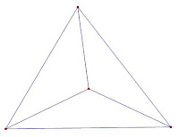
Solve this square system of 3 equations in 3 unknowns using your favorite method, and we find there is only one way to do this:

V = 4, E = 6 and R = 4.

The only solution is to have 4 triangles, 4 vertices and 6 edges as shown on the right, remembering that the outside region is a triangle.  So, we could never draw a graph that had 5 triangles such that 3 triangles meet at each vertex.  Give it a try to see why it can't be done.

Questions: Can we draw a planar graph of triangles where 4 triangles meet at each vertex? 5 triangles meet at each vertex? 6 triangles meet at each vertex? How would we change the system above to answer these questions.  If the graph exists, try to draw it. 

Example 2: What if there are two different types of polygons? Consider a graph of triangles and quadrilaterals, assuming that three polygons meet at each vertex. We will introduce two new variables: T and Q, the counts of the triangles and quadrilaterals, respectively. Now, the total number of regions is the sum of the two types of polygons,

T + Q = R.

Count the edges, 3 for each triangle and 4 for each quadrilateral, and as in Example 1, this counts each edge twice:

3T + 4Q = 2E.

Count the vertices, 3 for each triangle and 4 for each quadrilateral, and as in Example 1, this counts each vertex thrice, because 3 polygons meet at each vertex:

3T + 4Q = 3V.

Finally, we need the Euler Characteristic:

VE + R = 2.

This time we’ll use a matrix and row reduction to get the solution. The system is underdetermined, so we expect to get infinitely many solutions.


Sure enough, we have a free variable and we can write the general solution as

T = 12 – 2R,
Q = –12 + 3R,
V = –4 + 2R and
E = –6 + 3R.

But in this application, the values of T, Q, V and E have physical meaning and must be positive. If V or E is zero, then the graph would be empty. We could assume that T or Q is zero, but we are interested in graphs with both triangles and squares. Now we can solve the inequalities below to see if there is a viable solution, and how many there are.

T = 12 – 2R > 0      =>      R < 6
Q = –12 + 3R > 0      =>      R > 2
V = –4 + 2R > 0      =>      R > 2
E = –6 + 3R > 0      =>      R > 4

Okay, R is an integer and strictly between 4 < R < 6, so R = 5 is the only realistic solution to this underdetermined system. Now,

R = 5, T = 2, Q = 3, V = 6 and E = 9.

Draw this graph (don’t forget that the outside region is one of the 5 regions and must be either a quadrilateral or a triangle). The graph is at the bottom of this blog, but don’t peak before you give it a try.

Questions:

1. Can you draw a planar graph with pentagons and hexagons such that three polygons meet at each vertex? If so, how many of each polygon are there? Can you draw them?

2. Can you draw a planar graph with triangles and quadrilaterals such that four polygons meet at each vertex? I have written the equations and solved the system for this case, and this may have infinitely many solutions, but I haven’t had the time to draw more than two of the solutions and would like to see an algorithm for drawing all of them.

3. Other surfaces, such as a torus (donut) have different Euler Characteristics. How does one draw a graph on a torus? What are the solutions to the questions above if the graphs live on a torus?  Wolfram MathWorld has a list of the Euler Characteristics for surfaces, but WikiPedia has nice images of those surfaces if you scroll to the bottom of the article.

To limit this blog to a few pages, a lot is left unsaid. But again, these posts aren’t meant to give an in-depth discussion of the topic, but just an introduction.  Go exploring for more about this topic.

Reference: Alain M. Robert, An Approach of Linear Algebra through Examples and Applications